Intro to the Asymmetric Simple Exclusion Process (ASEP) & Bethe Ansatz Pt. 2
Published:
In this post I continue the discussion from this post on the ASEP and introduce the ‘Coordinate Bethe Ansatz’ approach to finding an explicit solution to the forward equation in the case of two particles. In part 1, we derived the following forward equation for the probability function of the ASEP,
\[\begin{split} \frac{d}{dt}u_Y(X;t) &= \sum_{i=1}^N p u(X_i^- ; t)\delta(x_{i-1} \neq x_{i} - 1) + q u(X;t)\delta(x_{i-1} \neq x_i - 1) \\ &- p u(X;t)\delta(x_{i+1}\neq x_i + 1) - q u(X;t)\delta(x_{i-1} \neq x_i - 1) \end{split}\]with initial condition \( u(X;0) = \delta(X=y) \). Now the approach we take will be as follows:
(1) Extend our domain to include equality of particle positions: \( \tilde{\mathcal{X}}_N(L) = { (x_1 \leq x_2 \leq \cdots \leq x_N ) }
(2) Split forward equation into a ‘free’ equation which describes particle dynamics with no interaction and a ‘boundary’ condition which ensures that we still obey the exclusion rule, i.e. when we project back into the original configuration space, we have equality with \( u(X;t) \)
(3) Establish an ansatz which solves the now much simpler free equation, satisfies the new boundary condition, and the initial condition.
This post will focus on the case of \( N = 2 \) particles, since it is the most constructive. First we consider \( u(X;t) \) with extended domain \( \tilde{\mathcal{X}} \). The two possible cases for the forward equation are illustrated below.
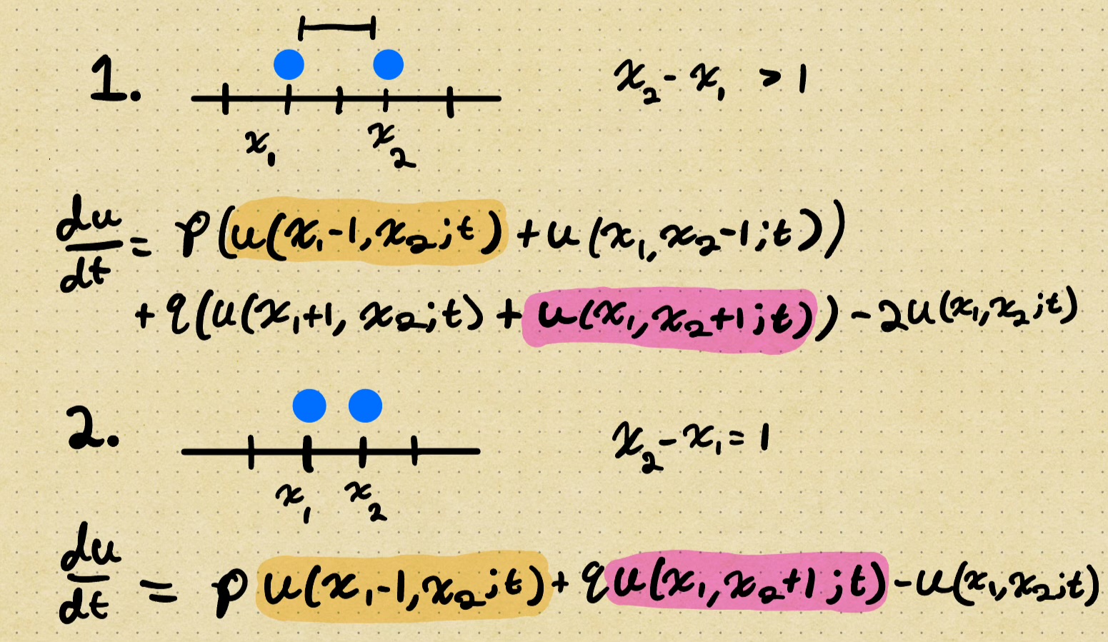
Subtracting (2) from (1) we obtain
\[0 = p u(x_1, x_2 - 1; t) + q u(x_1 + 1, x_2; t) - u(x_1, x_2; t)\]Which reads as
\[u(x, x+1; t) = p u(x, x; t) + q u(x + 1, x + 1; t)\]for \( x_2 = x_1 + 1 = x+1 \). This is our boundary condition, aptly named because it is an imposed equation on the boundary of the extended configuration space \( \tilde{\mathcal{X}} \). From case (1) in the illustration, we have our ‘free equation’
\[\frac{du}{dt} = \sum_{i=1}^2 p u(X_i^-; t) + q u(X_i^+; t) - u(X; t) = \sum_{i=1}^2 H_i u(X;t).\]We call this the free equation because it is the forward equation in the case where particles are not close enough to interact with each other. Now we move on to step 3, finding a solution to the free equation. Writing the right hand side in operator form with \( H_1 + H_2 = H \), we aim to find the eigenfunctions of \( H \) to get a general solution. That is, we want \( u(X;t) \) such that
\[\frac{du}{dt} = H u(X;t) = \lambda u(X;t)\]with \( \lambda \in \mathbb{C} \). Since \( H \) is only acting on the particle coordinates \( (x_1, x_2) \), we propose a separation of variables ansatz
\[u_Y(X;t) = \psi(X)\phi_Y(t)\]so then \( \phi_Y(t) = \alpha(Y) e^{\lambda t} \) if we can find \( \psi(X) \) such that \( H\psi(X) = \lambda \psi(X) \).
To find the proper form of solution for \( \psi \), we first inspect the eigenvalue equation in the case of a single particle:
\[H \psi(x) = p \psi(x-1) + q \psi(x + 1) - \psi(x) = \lambda \psi(x)\]This is a finite difference equation which has a general solution
\[\psi(x) = z^x\]for \( z \in \mathbb{C} \). Then,
\[p z^{x-1} + qz^{x+1} - z^x = \lambda z^x\]which gives us \( \lambda = pz^{-1} + qz - 1 \). For two particles, we can find the solution to
\[(H_1 + H_2)u(x_1, x_2; t) = \lambda u(x_1, x_2; t)\]in a similar manner where the ansatz of the difference equation is
\[\psi(x_1, x_2; t) = z_1^{x_1} z_2^{x_2} + A_{21} z_1^{x_2} z_2^{x_1}\]with \( z_1, z_2 \in \mathbb{C} \) and the eigenvalue becomes a sum of eigenvalues from the single particle case
\[\lambda = (pz_1^{-1} + qz_2 - 1) + (pz_2^{-1} + qz_2 -1) = \lambda_1 + \lambda_2.\]So for \( N = 2 \) we have eigenfunctions and eigenvalues for the free equation! So we’re done? Heck no! What is the coefficient \( A_{21} \)? What about \(z_1, z_2 \) ? And we can’t forget about \(\phi_Y(t)\), what is the coefficient \( \alpha(Y) \)? And we haven’t even touched the case of a general particle number \( N \). Luckily for us, we still have tools at our disposal that we haven’t used; namely the boundary condition, periodicity of the lattice, and initial condition. Stay tuned for part 3!