The Six-Vertex Model & XXZ Quantum Spin Chain part 2

Here we introduce the transfer matrix of the six-vertex model and show a mathematical relationship it has with the hamiltonian of the XXZ quantum spin chain (aka Heisenberg-Ising hamiltonian). This is a follow up to my previous blog post which you can find here. The work that follows is essentially that of section 10.14 in R.J. Baxter’s book “Exactly Solved Models in Statistical Mechanics” adapted to the more specific case of the six-vertex model and XXZ spin chain (compared to the more general XYZ spin chain and eight-vertex model).

The Transfer Matrix

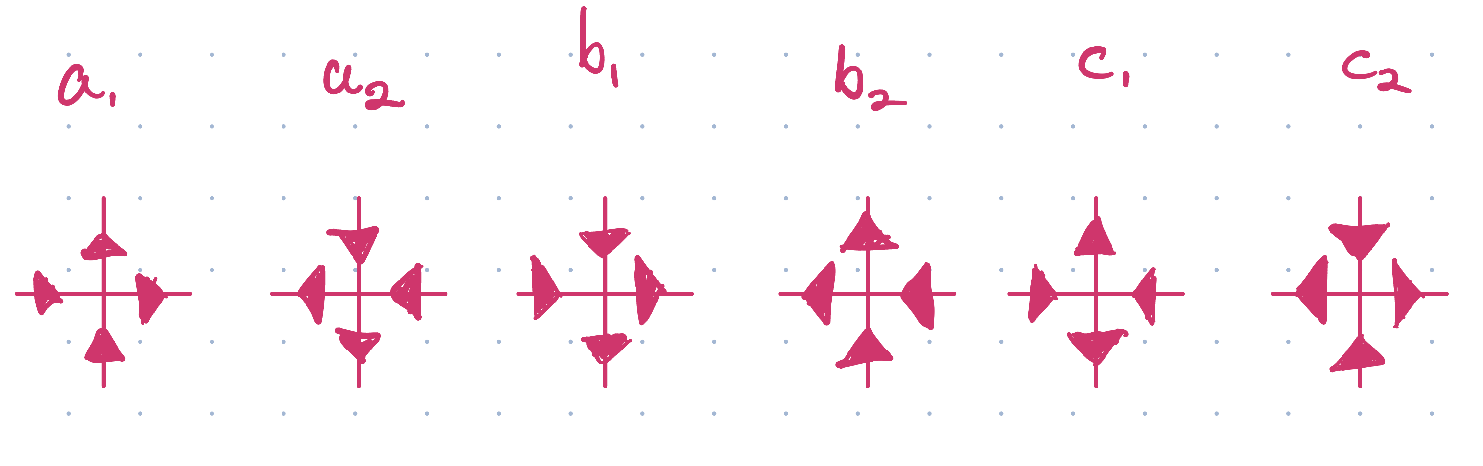
We first recall the arrow representation of the six possible vertex configurations. Moving forward these are the local configurations we will be referring to.

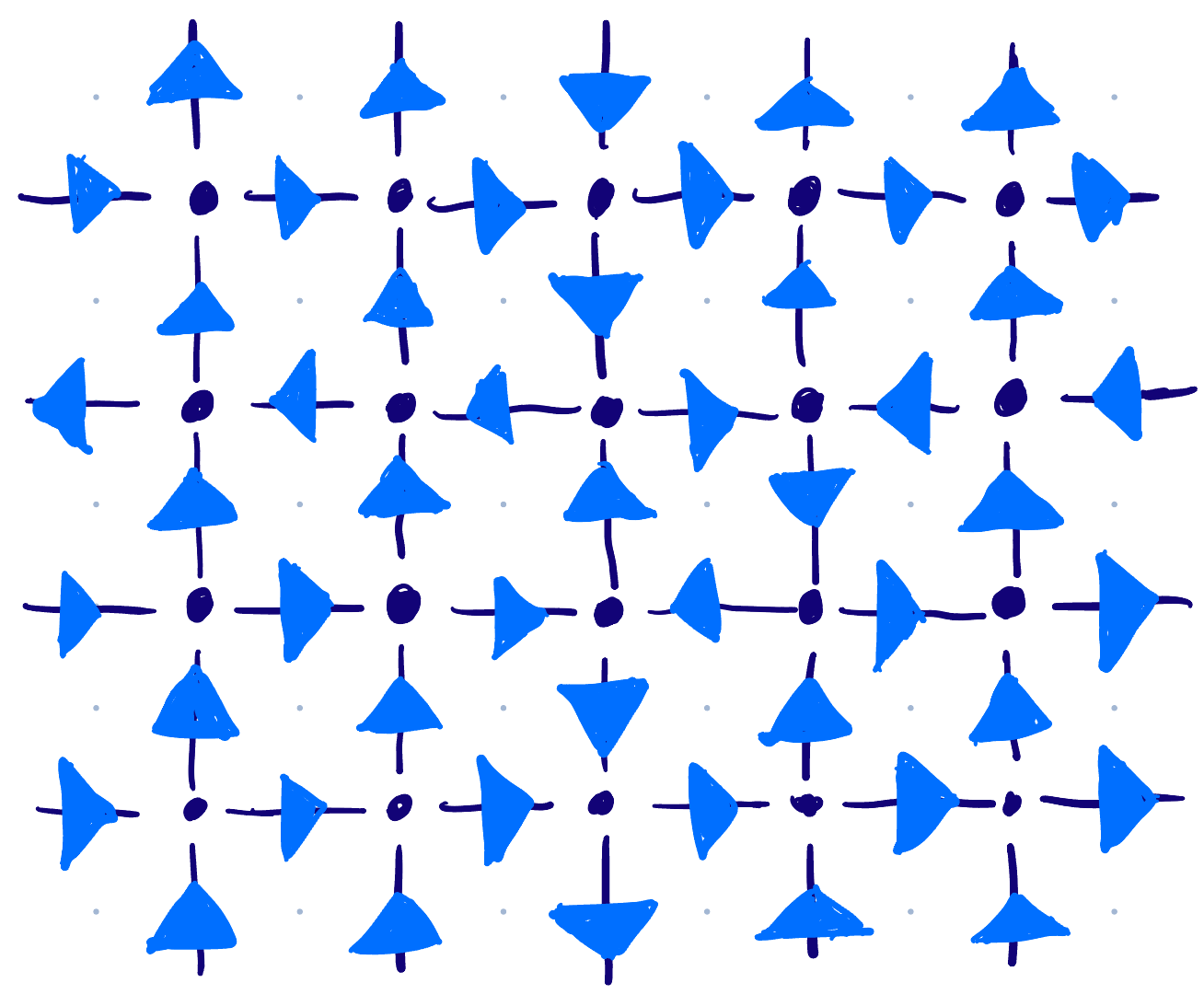
For a finite subset of our square lattice (let’s say M rows x N columns), we impose the ‘ice-rule’ which means for each vertex two of the adjacent arrows must point towards the vertex and two must point away from the vertex¹. This is what restricts us to the six local configurations. We will also impose toroidal boundary conditions which means the bottom & top edges and left & right edges are identified with each other respectively. Below is an example of a 4x5 configuration satisfying the ice-rule.

Now consider a horizontal row of the lattice and the adjacent horizontal and vertical edges. For each edge \(i\), associate a ‘spin’ (different from the quantum spin we consider in the XXZ spin chain) such that \(\mu_i=+1\) if the arrow is pointing up \((\uparrow)\) or to the right \((\rightarrow)\) and \(\mu_i=-1\) if the arrow is pointing down \((\downarrow)\) or to the left \((\downarrow)\). Let \(\mathbf{\alpha}=\{\alpha_1,\ldots,\alpha_N\}\) be the spins on the lower row of vertical edges, \(\mathbf{\beta}=\{\beta_1,\ldots,\beta_N\}\) be the spins on the upper row of vertical edges, and \(\mathbf{\mu}=\{\mu_1,\ldots,\mu_N\}\) be the spins on the horizontal edges. Note that the boundary conditions imply that \(\alpha_{N+1}=\alpha_1\) and similarly for \(\beta\) and \(\mu\). In terms of spins, we define the weights of local configurations in the following notation \(w(\mu, \alpha \mid \beta, \mu')\) where \(\mu\) is the horizontal arrow to the left of the vertex, \(\alpha\) is the vertical arrow below the vertex, \(\beta\) is the vertical arrow above the vertex, and \(\mu'\) is the horizontal arrow to the right of the vertex. Denoting \(+1\) spin value by \(+\) and \(-1\) spin value by \(-\), we have the local weights

where \(w=0\) otherwise. We define the transfer matrix \(V\) by is entries indexed by different spin configurations of vertical edge rows \(\mathbf{\alpha}\) and \(\mathbf{\beta}\) as follows

Where the transfer matrix meets the hamiltonian

In this section we will derive a direct relationship between the transfer matrix \(V\) and the XXZ hamiltonian \(\mathcal{H}\). Fix \(a=a_1=a_2\), \(b=b_1=b_2\), and \(c=c_1=c_2\). We can then rewrite the weight function \(w\) as

with \(a'=\frac12(a+b+c)\), \(b'=\frac12(a+b-c)\), and \(c'=\frac12(a-b+c)\). Equivalently,

where \(\delta(\alpha,\beta)=1\) if \(\alpha=\beta\) and zero otherwise (\(\delta\) here is the Kronicker delta). We will now compute a logarithmic derivative of \(V\) by varying the weights. First consider the case when \(b=0\) and \(a=c=c_0 > 0\). Then,

In this case we denote the transfer matrix as \(V_0\) and

which means that \(c_0^{-N} V_0\) is the left-shift operator sending the spin configuration \(\{\alpha_1,\ldots\alpha_N\}\) to \(\{\alpha_N,\alpha_1,\ldots,\alpha_{N-1}\}\). We can perturb this case setting \(a = c_0 + \delta a\), \(b=\delta b\), and \(c = c_0 + \delta c\) with \(\delta a\), \(\delta b\), \(\delta c\) infinitesemal increments in \(a, b, c\). Denote \(\delta w\) and \(\delta V\) as the increments induced in \(w\) and \(V\). Then

and then composing \(\delta V\) with \(V_0^{-1}\) we have \(\begin{equation} (V_0^{-1} \delta V)_{\mathbf{\alpha}\mathbf{\beta}}=c_0^{-1} \sum_{j=1}^N \cdots \delta(\alpha_{j-1},\beta_{j-1})\delta w(\alpha_j,\alpha_{j+1} \mid \beta_j,\beta_{j+1}) \delta(\alpha_{j+2},\beta_{j+2})\cdots. \end{equation}\)

We can rewrite this as a sum of operators if we define

so then

Up to this point one may have reasonably asked several times (if they kept reading that is) where the heck does the XXZ hamiltonian come into play? Fret not, this is where things begin to come together. Recall the hamiltonian \(\mathcal{H}\)

and spin operators \(S_j^x, S_j^y, S_j^z\). An alternative to the the tensor product definition of the spin operators, we can write \(\begin{equation} S_j^x = \frac{1}{\sqrt{2}}c_j, \quad S_j^y = \frac{1}{\sqrt{2}}i c_j s_j, \quad S_j^z = \frac{1}{\sqrt{2}}s_j \end{equation}\)

where

and

That is, \(s_j\) is a diagonal matrix with entries \(\alpha_j\) (the \(j\)‘th spin value (\(+1\) or \(-1\)) in the corresponding spin configuration \(\mathbf{\alpha}\)) and \(c_j\) is the spin-flip operator that reverses the spin in position \(j\). Now the relation between \(\mathcal{H}\) and \(V\) will appear via the operator \(U_j\), \(s_j\) and \(c_j\). We can express \(U_j\) in terms of \(s_j\) and \(c_j\) if write out the weight function \(w\) in \(U_j\)

and we can see that

So then

and thus

when \(\delta a = 0\) and \(\Delta = -\frac{\delta c}{2 \delta b}\). And hence with these parameters