An unexpected relationship: the mathematical ties of a model for a square sheet of ice and one-dimensional magnetism
Published:
What does a model for the possible orientations of hydrogen and oxygen atoms on a sheet of ice have to do with a toy model for magnetism on a chain? Although the original aim for both of these models were describing different things, molecular structure of ice and magnetism, they are intimately related via their mathematical construction. In particular, the operators that govern the dynamics of each model commute, and thus share the same eigenvectors.
XXZ Quantum Spin Chain & The Six Vertex Model
The following discussion and notes are based on the contents of 1,2,3,4. I encourage the interested reader to dive into these sources and the references therein for additional insight, rigor, and enjoyable mathematics.
XXZ Spin-1/2 Chain
Originally a toy model for magnetism, the XXZ Spin-1/2 chain describes a finite number of quantum spins on a 1D lattice (in our case a periodic lattice). The quantum spin at lattice site \( j \) in a chain of length \( L \) is described by the operators
\[\begin{equation*} \begin{split} S_j^\alpha &= \frac{1}{\sqrt{2}}\left(\mathrm{Id} \otimes\cdots \otimes \mathrm{Id} \otimes \sigma^{\alpha} \otimes \mathrm{Id} \otimes\cdots \otimes \mathrm{Id}\right) \\ \\ \sigma^x &= \begin{pmatrix} 0 & 1 \\ 1 & 0 \end{pmatrix},\quad \sigma^y = \begin{pmatrix} 0 & -i \\ i & 0 \end{pmatrix},\quad \sigma^z = \begin{pmatrix} 1 & 0 \\ 0 & -1 \end{pmatrix} \end{split} \end{equation*}\]which act on the L-fold tensor product, \(\mathbb{V}_L = \mathbb{V}^{\otimes L} \), of a 2D complex vector space with a basis given by spin up and down labels \(\mathbb{V}=\mathrm{Span}{ \mid \uparrow \rangle, \mid \downarrow \rangle } \). For example, the basis of $\mathbb{V}_2$ is given by \(\begin{equation*} \mid \uparrow \rangle \otimes \mid \uparrow \rangle = \mid \uparrow \uparrow \rangle,\, \mid \uparrow \rangle \otimes \mid \downarrow \rangle = \mid \uparrow \downarrow \rangle,\, \mid \downarrow \rangle \otimes \mid \uparrow \rangle = \mid \downarrow \uparrow \rangle,\, \mid \downarrow \rangle \otimes \mid \downarrow \rangle = \mid \downarrow \downarrow \rangle. \end{equation*}\) The \( \sigma^{\alpha} \) in \(S_j^\alpha \) is in the \( j \)’th position of the tensor product. The Hamiltonian operator, \( \mathcal{H} \), acts on elements of \( V_L \) (configurations of L spins) and its spectrum gives the energy levels of the system. The Hamiltonian for the XXZ spin-1/2 chain is defined as
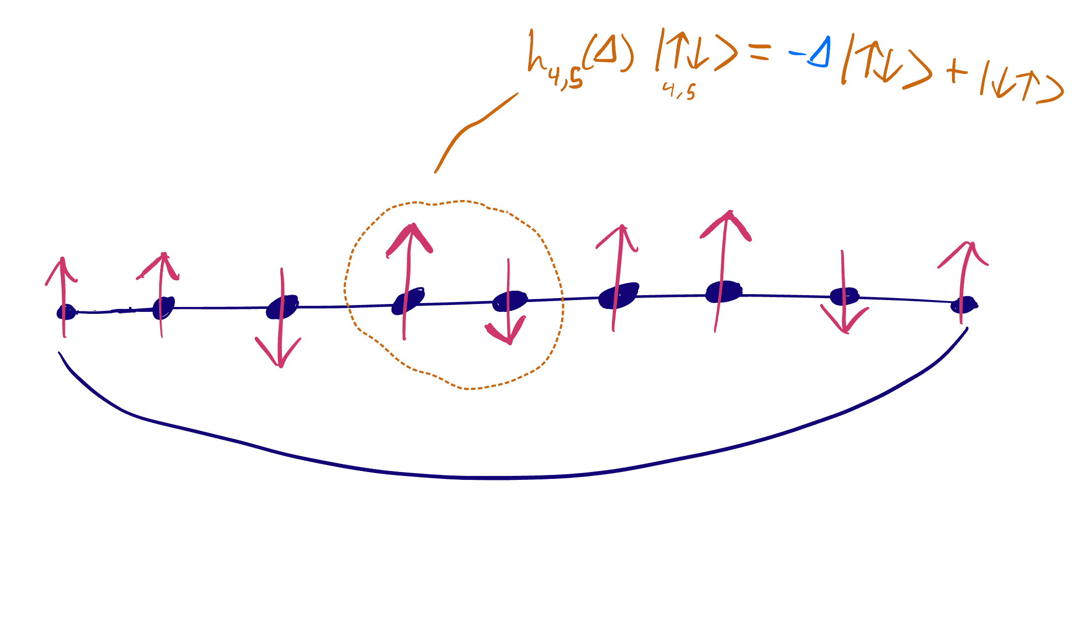
\[\begin{equation*} \begin{split} \mathcal{H} &= \sum_{i=1}^L h_{i,i+1}(\Delta) \\ h_{i,i+1}(\Delta) &= S_i^x S_{i+1}^x + S_i^y S_{i+1}^y + \Delta( S_i^z S_{i+1}^z - 1/2) = \mathrm{Id} \otimes\cdots\otimes \begin{pmatrix} 0 & 0 & 0 & 0 \\ 0 & -\Delta & 1 & 0 \\ 0 & 1 & -\Delta & 0 \\ 0 & 0 & 0 & 0 \end{pmatrix} \otimes \cdots \mathrm{Id} \end{split} \end{equation*}\]with \(\Delta\in\mathbb{R}\). A property of great importance is that the local operator \(h_{i,i+1}(\Delta)\) conserves the number of up-spins (consequently also the down-spins) and hence the hamiltonian \(\mathcal{H}\) also conserves the number of up/down-spins. It is a nice exercise to check this property if you are unfamiliar with spin chains (note that the four columns/rows in the matrix of the \(i\) and \(i+1\) locations in the tensor product of \(h_{i,i+1}\) correspond to \(\mid \uparrow\uparrow \rangle, \mid \uparrow\downarrow \rangle, \mid \downarrow\uparrow \rangle, \mid \downarrow\downarrow \rangle\) in that order which are the basis vectors of the \(i\) and \(i+1\) neighboring spins). This conservation of spin leads us to consider subspaces of \(V_L\) which correspond to a fixed number of up-spins \(N\) (\(L-N\) down-spins). Here is a quick illustration of a chain of length \(L=9\) and number of up-spins \(N=6\) with an example of the local operator for the 4th and 5th spin sites.
Six-Vertex Model
Originally introduced to compute numerical characteristics of ice, the six-vertex model consists of a square lattice (\(\mathbb{Z}^2\)) whose vertices represent oxygen atoms and edges represent hydrogen atoms. Since H\(_2\)0 contains two H atoms and one oxygen atom, a configuration is when each O atom is matched with exactly two neighboring H atoms. On a square lattice, this leads to six possible local configurations (hence the “six-vertex” in the name) illustrated below.
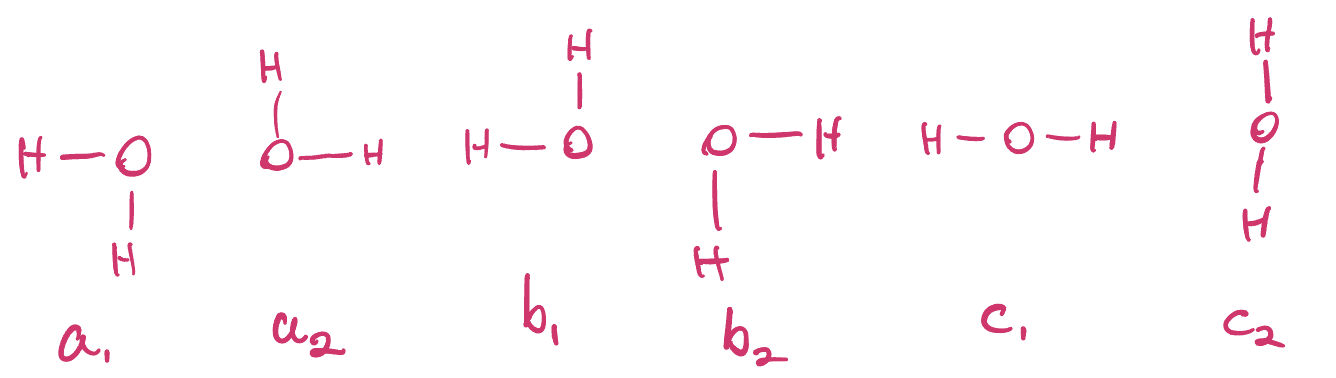
For each local configuration, we assign a weight denoted \(a_1, a_2, b_1, b_2, c_1,\) or \(c_2\) which you can see labeled above. If we restrict to a finite subset of the infinite square lattice \(\mathbb{Z}\), the configuration space is comprised of local configurations assigned to the vertices which are consistent with each other. For example:
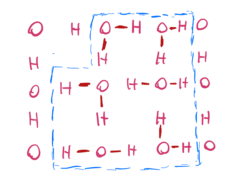
For a configuration/state \(S\), we assign the probability
\[\begin{equation*} Prob(S)=\frac1Z \prod_{(i,j)} weight(i,j;S) \end{equation*}\]where \(Z\) is the normalization constant, called the partition function, and the product is over all vertices \((i,j)\) in the finite subset of the lattice. For instance, the state in the above example has the following probability:
\[\begin{equation*} \frac1Z (b_2 \cdot b_2 \cdot a_1 \cdot c_1 \cdot c_1 \cdot a_2) = \frac1Z a_1 \cdot a_2 \cdot b_2^2 \cdot c_1^2 \end{equation*}\]Notice that \(Prob(S)\) can also be written as
\[\begin{equation*} \frac1Z (a_1^{n(a_1)}\cdot a_2^{n(a_2)} \cdot b_1^{n(b_1)} \cdot b_2^{n(b_2)} \cdot c_1^{n(c_1)} \cdot c_2^{n(c_2)}) \end{equation*}\]where \(n(v)=\) #vertices of type \(v\).
Another representation of six-vertex configurations
Since the hydrogen-ion bonds form electric dipoles, we can represent the local configurations with arrows pointing towards the vertex if an H atom is present and away from the vertex otherwise (see illustration below).
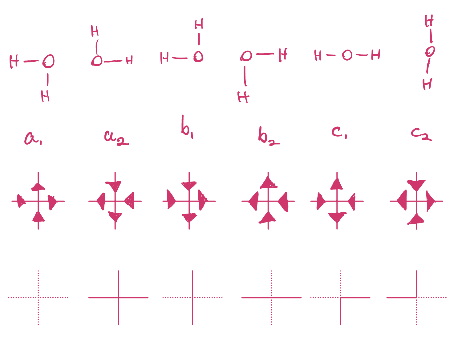
Moreover, we can represent local configurations with lines present if arrows are pointing down or to the left which is the third row of pictures you see above. This last representation gives a nice interpretation of configurations as up-right paths in the square lattice. A priori it is not entirely clear by its construction how the six-vertex model relates to the XXZ spin chain. In the next blog posts we will introduce the transfer matrix, \(\mathcal{V}\), for the six-vertex model and uncover that the XXZ Hamiltonian, \(\mathcal{H}\), is effectively a logarithmic derivative of \(\mathcal{V}\). Stay tuned!
R. J. Baxter, “Exactly Solved Models in Statistical Mechanics” Academic Press, 1982 Copyright: Rodney J. Baxter 2004 ↩
https://www.ams.org/journals/bull/2025-62-02/S0273-0979-2025-01846-7/S0273-0979-2025-01846-7.pdf ↩
https://arxiv.org/pdf/1611.09909 ↩
John Parkinson, Damian J J Farnell, “An Introduction to Quantum Spin Systems” Springer-Verlag Berlin Heidelberg 2010 ↩