Intro to the Asymmetric Simple Exclusion Process (ASEP) Pt. 1
Published:
A brief introduction to the asymmetric simple exclusion process (ASEP) and the forward equation for the dynamics.
The Asymmetric Simple Exclusion Process
Consider a chain of particles on a discrete ring (see figure 1) which move left and right with probabilities \(q\) and \(p\), respectively, with \(p+q=1.\) Each particle on its own is a random walker, but what happens when two particles encounter the same lattice site? In defining this model, one can come up with several different kinds of interaction rules. Perhaps a particle moving into the occupied site is a bully and pushes the occupying particle over into the neighboring site. Maybe the particles coexist and sit together on the same site. It could be that the particles merge into a single particle. The possibilities are endless, with each yielding its own unique set of questions. In this post, we will be discussing a simple exclusion process, where a particle is prevented from moving into an occupied site. In particular, our jumping rates will be unequal (\(p\neq q\)), giving us the name: the Asymmetric Simple Exclusion Process (ASEP).
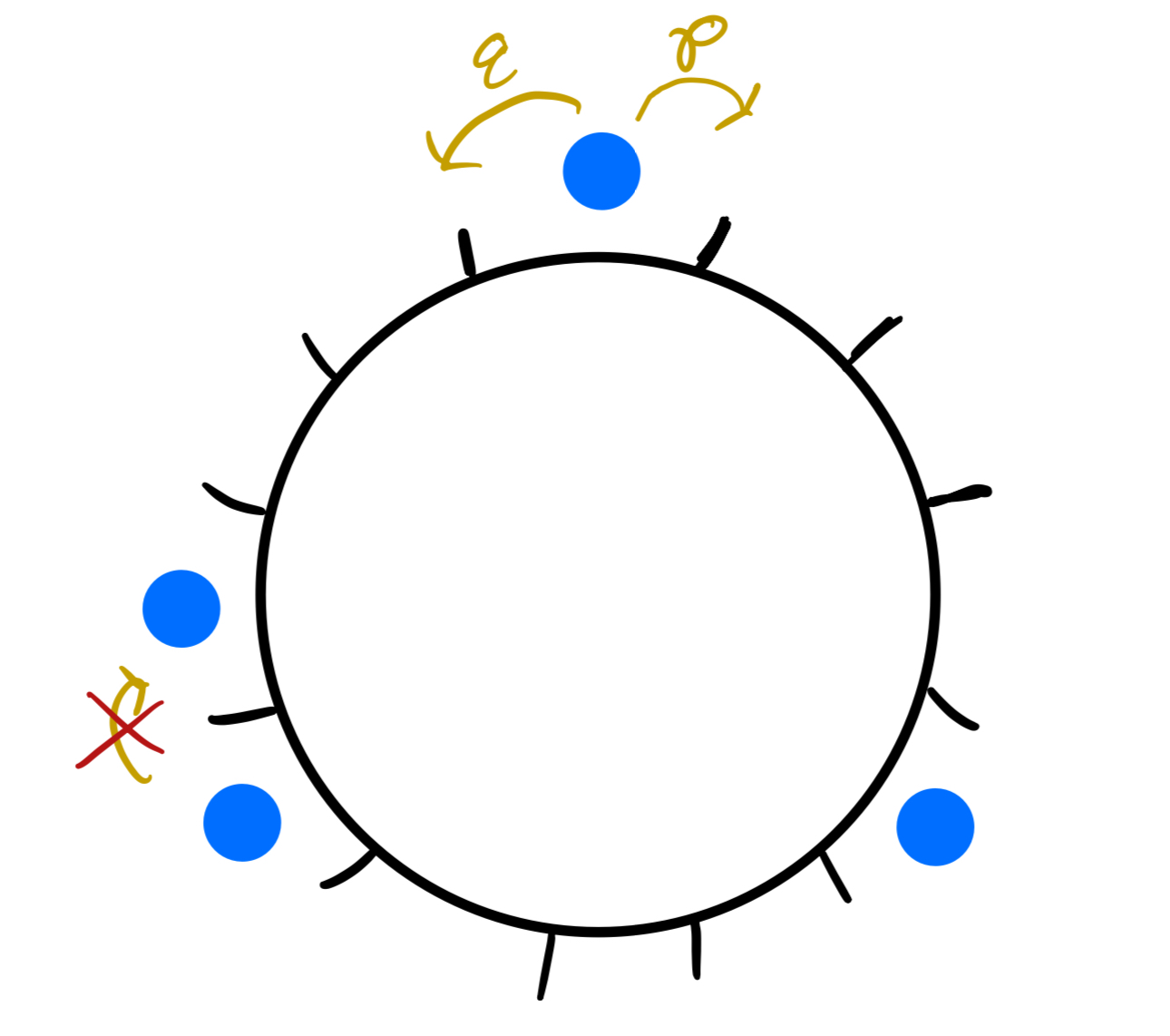 Figure 1: ASEP on a ring with 12 sites and 4 particles.
While the relatively easy-to-describe rules governing ASEP are lovely, it’s widely known that a many-body system with simple local rules is not always amenable to achieving exact mathematical expressions which can fully describe the system. Describing the system in the sense that for a random process we’d like to answer questions regarding its underlying probability distribution. Moreover, we’d like to understand the asymptotics of the system. What happens to the system after a really long period of time? When the size of the lattice and number of particles get infinitely large? Answering these questions may provide evidence (or better yet, mathematical proof) that there is some kind of universality driving the behavior of the macroscopic system that bears no resemblance to the microscopic rules which define it. And if this is the case, does it yield the same universal behavior as other models which seemingly describe entirely different systems? While addressing these questions may not be easy, finding analytical1 formulas for the model provides a first step towards asymptotics.
In ASEP, with \(N\) particles and \(L\) sites, our state space is
\[\begin{equation*} \mathcal{X}_N(L) = \{ (x_1,\ldots,x_N) \in (\mathbb{Z}/L\mathbb{Z})^N : x_1, \ldots, x_N \text{ has strict increasing cyclic order} \} \end{equation*}\]where \(x_i\) denotes the location of the \(i\)’th particle. Our dynamics are governed by the forward equation
\[\begin{equation*} \begin{split} \frac{d}{dt}u_Y(X;t) = \sum_{i=1}^{N}&pu_Y(X_i^-;t)\delta(x_i \neq x_{i-1}+1) + qu_Y(X_i^-;t)\delta(x_i \neq x_{i+1} - 1) \\ - &pu_Y(X_i;t)\delta(x_i\neq x_{i+1}-1) - qu_Y(X_i;t)\delta(x_i \neq x_{i-1}+1) \end{split} \end{equation*}\]where \(Y=(y_1,\ldots,y_N)\) denotes the intial configuration of particles, \ \(X_i^{\pm} = (x_1,\ldots,x_{i-1},x_i\pm1,x_{i+1},\ldots,x_N) \), equality in the indicator functions, \delta, is modulo \(L\), and \(u_Y(X;t) = \mathbb{P}_Y(X;t)\) is the probability of configuration \(X\) at time \(t\). With the initial condition
\[\begin{equation} u_Y(X;0)=\delta(X=Y), \hspace{0.25cm} \forall X\in\mathcal{X}_N(L), \end{equation}\]\(u_Y(X;t)\) is uniquely determined by the forward equation. To construct the forward equation, knowing that the recipe for the forward equation is
\[\frac{d}{dt}Prob(\text{state }x;t) = \text{Prob. going into state }x - \text{Prob. going out of state }x\]is quite helpful. Let’s take a look at how this construction works.
Constructing the forward equation
If we focus on the dynamics of a single particle, there are only two ways that a particle can be prevented from jumping: either it has a neighboring particle on the left, or it has a neighboring particle on the right. So our probability of moving into an arbitrary state \( X=(x_1,\ldots,x_i,\ldots,x_N) \) when particle \( i \) jumps is the probability of it jumping right \( p u(X_i^- ; t)\delta(x_{i-1} \neq x_{i} - 1) \) and jumping left \( q u(X_i^+ ; t)\delta(x_{i+1}\neq x_i + 1) \) with the conditions that in state \( X \) there is not a particle directly to the left or right of the \( i \)’th particle.
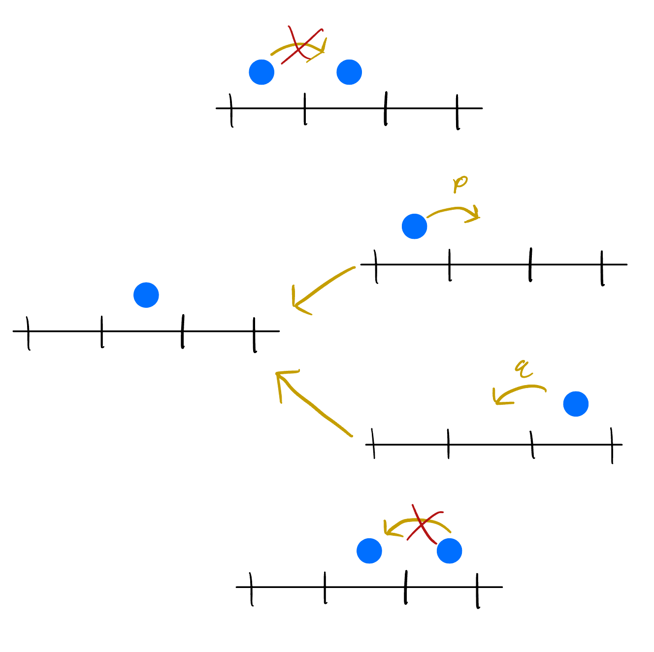
Figure 2: The possible cases where the system can move into state \( X \) and the exclusion conditions are marked with a red x on the jump arrow.
Similarly, our probability of moving out of an arbitrary state \( X \) when the \( i \)’th particle jumps is the probability of it jumping left \( q u(X;t)\delta(x_{i-1} \neq x_i - 1) \) and jumping right \( p u(X;t)\delta(x_{i+1}\neq x_i + 1) \) provided there aren’t particles blocking it to the left and right, respectively.
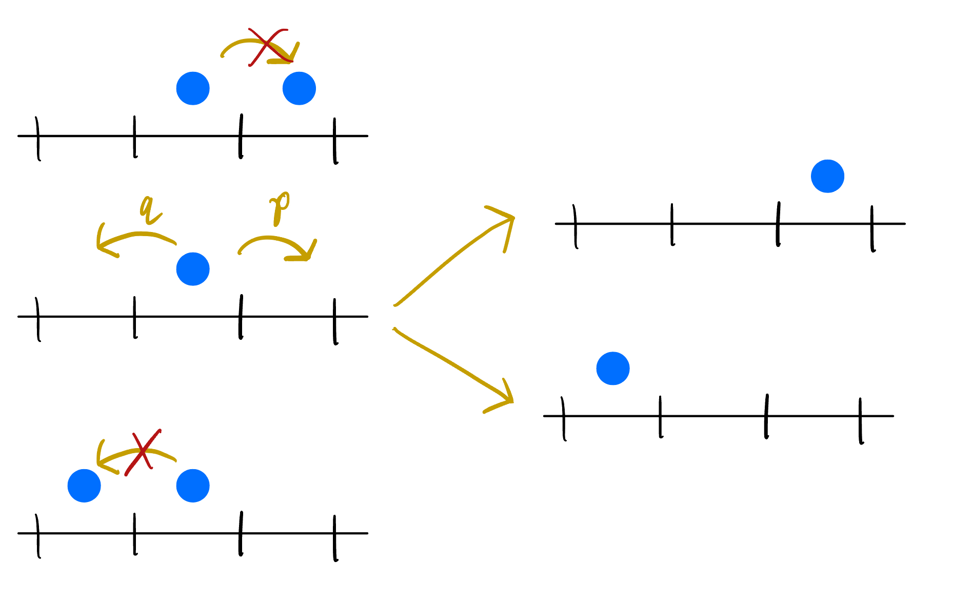
Figure 3: The possible cases where the system can move out of state \( X \) with exclusion conditions.
So following our probability in \( - \) probability out formula for the forward equation, we get
\[\begin{split} \frac{d}{dt}u_Y(X;t) &= \sum_{i=1}^N p u(X_i^- ; t)\delta(x_{i-1} \neq x_{i} - 1) + q u(X;t)\delta(x_{i-1} \neq x_i - 1) \\ &- p u(X;t)\delta(x_{i+1}\neq x_i + 1) - q u(X;t)\delta(x_{i-1} \neq x_i - 1) \end{split}\]where the sum is over all \( N \) particles. Now, if we can solve the forward equation exactly and satisfy the initial condition, then we have the unique probability function which describes our entire system. To do this, though, we will use an equivalent formalism which splits our forward equation into a ‘free’ part which contains the non-interaction of particles, and a ‘boundary’ condition which contains the interacting component. This will lead us to the famous Bethe Ansatz, which will be described in part 2!
Analytical in the sense that we can do things with it like take limits ↩